EMC Software

Introduction

As part of our collaboration with the OMAC User's Group, we have written software which implements real-time control of equipment such as machine tools, robots, and coordinate measuring machines. The goal of this software development is twofold: first, to provide complete software implementations of all OMAC modules for the purpose of validating application programming interfaces; and second, to provide a vehicle for the transfer of control technology to small- and medium-sized manufacturers via the NIST Manufacturing Extension Partnership.

The EMC software is based on the NIST Real-time Control System (RCS) Methodology, and is programmed using the NIST RCS Library. The RCS Library eases the porting of controller code to a variety of Unix and Microsoft platforms, providing a neutral application programming interface (API) to operating system resources such as shared memory, semaphores, and timers. The RCS Library also implements a communication model, the Neutral Manufacturing Language, which allows control processes to read and write C++ data structures throughout a single homogeneous environment or a heterogeneous networked environment.

The EMC software is written in C and C++, and has been ported to the PC Linux, Windows NT, and Sun Solaris operating systems. When running actual equipment, a real-time version of Linux is used to achieve the deterministic computation rates required (200 microseconds is typical). The software can also be run entirely in simulation, down to simulations of the machine motors. This enables entire factories of EMC machines to be set up and run in a computer integrated manufacturing environment. A Windows NT simulation self-installing archive runs the controller on simulated DC motors, with a Java GUI.

The EMC software is available free of charge on our FTP site. Please read the README file before getting or installing the software.

This software was prepared by United States Government employees as part of their official duties and is, therefore, a work of the U.S. Government and not subject to copyright.

The EMC at Work

EMCs have been installed on many machines, both with servo motors and stepper motors. Here is a sampling:

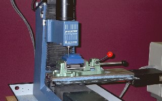
3-axis Bridgeport knee mill at Shaver Engineering. The machine uses DC brush servo motors and encoders for motion control, and OPTO-22 compatible I/O interfaced to the PC parallel port for digital I/O to the spindle, coolant, lube, and estop systems.
	3-axis desktop milling machine used for prototype development. The machine uses DC brush servo motors and encoders. Spindle control is accomplished using the 4th motion control axis. The machine cuts wax parts.
4-axis Kearney & Trecker horizontal machining center at General Motors Powertrain in Pontiac, MI. This machine ran a precursor to the full-software EMC which used a hardware motion control board.

EMC Components

There are four components to the EMC software: a motion controller (EMCMOT), a discrete I/O controller (EMCIO), a task executor which coordinates them (EMCTASK), and a collection of text-based or graphical user interfaces.

Graphical User Interfaces

The EMC comes with several types of user interfaces: an interactive command-line program emcpanel, a character-based screen graphics program keystick, an X Windows program xemc, a Java-based GUI emcgui, and a Tcl/Tk-based GUI TkEmc.

TkEmc is most well-supported, and runs on Linux and Microsoft Windows. The Windows version can connect to a real-time EMC running on a Linux machine via a network connection, allowing the monitoring of the machine from a remote location. TkEmc comes with the Linux distribution of the EMC. Instructions for installing and configuring the Windows version can be found in wintkemc.html.

Motion Controller EMCMOT

The motion controller (Figure 1) is written in C for maximum portability to real-time operating systems. Motion control includes sampling the position of the axes to be controlled, computing the next point on the trajectory, interpolating between these trajectory points, and computing an output to the motors. For servo systems, the output is based on a PID compensation algorithm. For stepper systems, the calculations run open-loop, and pulses are sent to the steppers based on whether their accumulated position is more than a pulse away from where their commanded position should be.

The motion controller includes programmable software limits, interfaces to hardware limit and home switches, PID servo compensation with zero, first, and second order feedforward, maximum following error, selectable velocity and acceleration values, individual axis jogging (continuous, incremental, absolute), queued blended moves for linear and generalized circular motion, and programmable forward and inverse kinematics.

The motion controller is written to be fairly generic. Initialization files (with the same syntax as Microsoft Windows INI files) are used to configure parameters such as number and type of axes (e.g., linear or rotary), scale factors between feedback devices (e.g., encoder counts) and axis units (e.g., millimeters), servo gains, servo and trajectory planning cycle times, and other system parameters. Complex kinematics for robots can be coded in C according to a prescribed function interface and linked in to replace the default 3-axis Cartesian machine kinematics routines. A C language application programming interface (API) between the motion controller and the external world is provided so that specific hardware can be integrated into the EMC without modifying any of the core control code. Programmers must implement these API functions for each board.

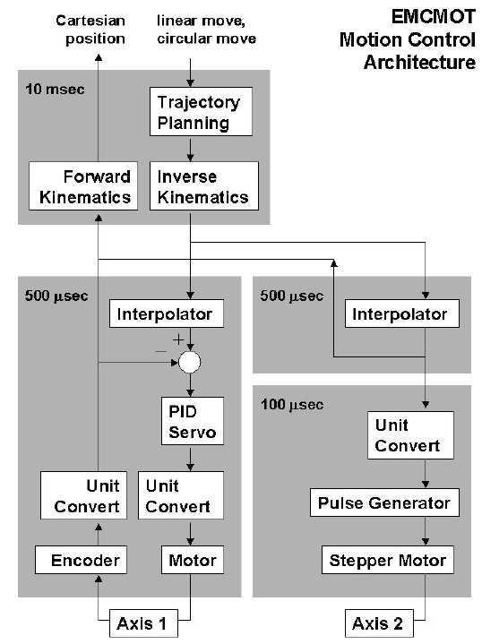
Figure 1. Motion controller software architecture. This figure shows two axes of control, with axis 1 using a servo motor and axis 2 using a stepper motor. For steppers, the commanded position is feed back directly as the motor position, so the system operates open-loop. A second task compares the output position with the accumulated pulse count, and generates a pulse if the difference is greater than half the pulse distance. The motion controller is a single C program, executing cyclically. When controlling actual machines, the motion controller requires a real-time operating system. In our installations, we have used RT-Linux. This gives real-time deterministic cycle times down to about 100 microseconds. The motion controller uses either shared memory or RT-Linux FIFOs to receive commands or send status, error, or logging information. NML is not used directly by the motion controller since NML requires C++ and the coding was limited to C to maximize portability to other real-time operating systems.

Setting up Stepper Motors

Currently the EMC supports stepper motors with a 2-bit step-and-direction interface, with bits mapped to the parallel port. Each parallel port has 12 bits of output and 5 bits of input. The outputs are used to drive the step and direction of each motor. 12 bits of output mean that up to 6 stepper motors can be controlled. The inputs can be used to detect limit or home switch trips. 5 bits of input mean that only one axes can get full positive, negative, and home switch inputs. The EMC mapping compromises for 3 axes of stepper motor control, with all positive limit switches being mapped to one input, all negative limit switches being mapped to another input, and all home switches being mapped to a third input. Other permutations are possible, of course, and can be changed in the software. You could also add 2 additional parallel ports (LPT2, LPT3), and get 36 bits of output and 15 bits of input. Some parallel ports also let you take 4 outputs and use them as inputs, for 8 outputs and 9 inputs for each parallel port. This would let you get 3 axes of control and full switch input per parallel port. See Using the PC parallel port for digital I/O for more information on the parallel port.

The pinout for the EMC stepper motor interface is as follows:

Output        Parallel Port
------        -------------
X direction   D0, pin 2
X clock       D1, pin 3
Y direction   D2, pin 4
Y clock       D3, pin 5
Z direction   D4, pin 6
Z clock       D5, pin 7

Input         Parallel Port
-----         -------------
X/Y/Z lim +   S3, pin 15
X/Y/Z lim -   S4, pin 13
X/Y/Z home    S5, pin 12

Stepper motor control is implemented using a second real-time task that runs at 100 microseconds. This task writes the parallel port output with bits set or cleared based on whether the a pulse should be raised or lowered. This gives an effective period of 200 microseconds for a full up-and-down pulse, or a 5 kilohertz frequency.

Discrete I/O Controller EMCIO

The discrete I/O controller (bottom right in Figure 2) is written in C++, using the NIST RCS Library. It is based on a hierarchy of C++ controller classes derived from the NML_MODULE base class, each communicating using NML. Discrete I/O controllers are highly machine-specific, and are not customizable in general using the INI file technique used to configure the more generic motion controller.

A C language application programming interface (API) between the discrete I/O controller and the external world is provided so that specific hardware can be integrated into the EMC without modifying any of the core control code. Programmers must implement these API functions for each board.

Task Executor EMCTASK

The Task Executor (at the top in Figure 2) is coded similarly to the discrete I/O controller, using the NML_MODULE base class and the RCS Library. It is less machine specific than the discrete I/O controller, as it is responsible for interpreting G and M code programs whose behavior does not vary appreciably between machines.

External Programs

Indicated at the very top in Figure 2 is the fourth component of the EMC software, the external programs such as the graphical user interface (GUI) or flexible manufacturing system (FMS) which are used to run the EMC. These communicate using NML, sending messages such as power on, enter automatic mode, run a program, or power down. GUIs may send manual commands initiated by the operator, for example jogging machine axes in manual mode, or homing each axis.

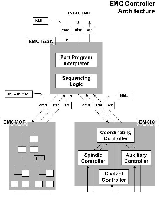
Figure 2. EMC controller software architecture. At the coarsest level, the EMC is a hierarchy of three controllers: the task level command handler and program interpreter, the motion controller, and the discrete I/O controller. The motion controller is detailed in Figure 1. The discrete I/O controller is implemented as a hierarchy of controllers, in this case for spindle, coolant, and auxiliary (e.g., estop, lube) subsystems. The task controller coordinates the actions of the motion and discrete I/O controllers. Their actions are programmed in conventional numerical control "G and M code" programs, which are interpreted by the task controller into NML messages and sent to either the motion or discrete I/O controllers at the appropriate times.

Configuring the EMC

The EMC is configured with files that are read at startup and used to override the compiled defaults. No real controller will likely use the compiled defaults, so you will certainly need to edit at least some of these files to reflect the specifics of your machine.

There are four files: emc.ini, emc.nml, tool.tbl, and rs274ngc.var. The first, emc.ini, contains all the machine parameters such as servo gains, scale factors, cycle times, units, etc. and will certainly need to be edited. emc.nml contains communication settings for shared memory and network ports you may need to override on your system, although it is likely that you can leave these settings alone. tool.tbl contains the tool information such as which pocket contains which tool, and the length and diameter for each tool. rs274ngc.var contains variables specific to the RS-274-NGC dialect of NC code, notably for setting the persistent numeric variables for the nine work coordinate systems. The specific formats of each of these files is detailed in the following sections.

Machine Configuration file emc.ini

[SECTION]

; COMMENT
SYMBOL = VALUE

You can edit the values for each keyword in any text editor. The changes won't take effect until the next time the controller is run. The file should be called emc.ini, but the name can be overriden using a command line argument to the controllers. See the section "Starting Up" for information on how to do this. The following sections detail each section of the configuration file, using sample values for the configuration lines.

[EMC] Section

• VERSION = $Revision: 1.14 $

  The version number for the INI file. This is automatically updated when using the Revision Control System, which looks for the $Revision: 1.14 $ string and appends the revision number. If you want to edit this manually just change the number and leave the other tags alone.

• MACHINE = My Controller

  This is the name of the controller, which is printed out when it runs. You can put whatever you want here.

[TASK] Section

• CYCLE_TIME = 0.100

  The period, in seconds, at which EMCTASK will run. You can make this as small as you want to increase the throughput. Making it 0.0 or a negative number will tell EMCTASK not to sleep at all. Ultimately the system loading will limit the effective throughput.

[TRAJ] Section

The [TRAJ] section contains general parameters for the trajectory planning module in EMCMOT.

• AXES = 3

  The number of controlled axes in the system.

• LINEAR_UNITS = 0.03937007874016

  The number of linear units per millimeter. For systems executing in native English (inch) units, this value is as shown above. For systems executing in native millimeter units, this value is 1. This does not affect the ability to program in English or metric units in NC code. It is used to determine how to interpret the numbers reported in the controller status by external programs.

• ANGULAR_UNITS = 1.0

  The number of angular units per degree. For systems executing in native degree units, this value is as shown above. For systems executing in radians, this value is 0.01745329252167, or PI/180.

• CYCLE_TIME = 0.010

  The period in seconds at which trajectory calculations are performed. This is a multiple of the period at which servo calculations are performed, as set in the [AXIS_#] CYCLE_TIME entry. Trajectory calculations are called at multiples of the servo period to plan linear or circular motion in Cartesian space. These values are interpolated at the servo period and run through the inverse kinematics.

• DEFAULT_VELOCITY = 1.0

  The initial velocity used for axis or coordinated axis motion, in user units per second.

• DEFAULT_ACCELERATION = 100.0

  The initial acceleration used for axis or coordinated acis motion, in user units per second per second.

• MAX_VELOCITY = 5.0

  The maximum velocity for any axis or coordinated move, in user units per second.

• MAX_ACCELERATION = 100.0

  The maximum acceleration for any axis or coordinated axis move, in user units per second per second.

[AXIS_#] Sections

The [AXIS_0], [AXIS_1], etc. sections contains general parameters for the individual axis control modules in EMCMOT. The axis section names begin numbering at 0, and run through the number of axes specified in the [TRAJ] AXES entry minus 1.

• TYPE = LINEAR

  The type of axes, either LINEAR or ANGULAR. Values for the position of LINEAR axes are in the units (per millimeter) specified in the [AXIS_#] UNITS entry. Values for the position of ANGULAR axes are in the units (per degree) specified in the same entry.

• UNITS = 0.03937007874016

  Units per millimeter for a LINEAR axis, as defined in the [AXIS_#] TYPE section, or units per degree for an ANGULAR axis as defined in the same section.

• P = 50

  The proportional gain for the axis servo. This value multiplies the error between commanded and actual position in user units, resulting in a contribution to the computed voltage for the motor amplifier. The units on the P gain are volts per user unit.

• I = 0

  The integral gain for the axis servo. The value multiplies the cumulative error between commanded and actual position in user units, resulting in a contribution to the computed voltage for the motor amplifier. The units on the I gain are volts per user unit-seconds.

• D = 0

  The derivative gain for the axis servo. The value multiplies the difference between the current and previous errors, resulting in a contribution to the computed voltage for the motor amplifier. The units on the D gain are volts per user unit per second.

• FF0 = 0

  The 0-th order feedforward gain. This number is multiplied by the commanded position, resulting in a contribution to the computed voltage for the motor amplifier. The units on the FF0 gain are volts per user unit.

• FF1 = 0

  The 1st order feedforward gain. This number is multiplied by the change in commanded position per second, resulting in a contribution to the computed voltage for the motor amplifier. The units on the FF1 gain are volts per user unit per second.

• FF2 = 0

  The 2nd order feedforward gain. This number is multiplied by the change in commanded position per second per second, resulting in a contribution to the computed voltage for the motor amplifier. The units on the FF2 gain are volts per user unit per second per second.

• CYCLE_TIME = 0.001

  This is the period in seconds at which servo calculations will run. The values can be different between different axes, and the lowest will be used for all. This ensures that the calculations will occur at least as fast as they are specified here. The value should be an integer submultiple of the trajectory cycle time specified in the [TRAJ] CYCLE_TIME entry, so that an integer number of interpolations will occur. If this is not the case the times will be forced so that the interpolation interval is the next highest integer.

• INPUT_SCALE = 40000 0

  These two values are the scale and offset factors for the axis input from the raw feedback device, e.g., an incremental encoder. The second value (offset) is subtracted from raw input (e.g., encoder counts), and divided by the first value (scale factor), before being used as feedback. The units on the scale value are in raw units (e.g., counts) per user units (e.g., inch). The units on the offset value are in raw units (e.g., counts).

  Specifically, when reading inputs, the EMC first reads the raw sensor values. The units on these values are the sensor units, typically A/D counts, or encoder ticks. These units, and the location of their 0 value, will not in general correspond to the quasi-SI units used in the EMC. Hence a scaling is done immediately upon sampling:

    input = (raw - offset) / scale
  

  The value for scale can be obtained analytically by doing a unit analysis, i.e., units are [sensor units]/[desired input SI units]. For example, on a 2000 counts per rev encoder, and 10 revs/inch gearing, and desired units of mm, we have

    [scale units] = 2000 [counts/rev] * 10 [rev/inch] * 1/25.4 [inch/mm]
                  = 787.4 counts/mm
  

  and, as a result,

    input [mm] = (encoder [counts] - offset [counts]) / 787.4 [counts/mm]
  

  Note that the units of the offset are in sensor units, e.g., counts, and they are pre-subtracted from the sensor readings. The value for this offset is obtained by finding the value of counts for which you want your user units to read 0.0. This is normally accomplished automatically during a homing procedure.

• OUTPUT_SCALE = 1 0

  These two values are the scale and offset factors for the axis output to the motor amplifiers. The second value (offset) is subtracted from the computed output (in volts), and divided by the first value (scale factor), before being written to the D/A converters. The units on the scale value are in true volts per DAC output volts. The units on the offset value are in volts. These can be used to linearize a DAC.

  Specifically, when writing outputs, the EMC first converts the desired output in quasi-SI units to raw actuator values, e.g., volts for an amplifier DAC. This scaling looks like:

    raw = (output - offset) / scale
  

  The value for scale can be obtained analytically by doing a unit analysis, i.e., units are [output SI units]/[actuator units]. For example, on a machine with a velocity mode amplifier such that 1 volt results in 250 mm/sec velocity, we have:

    [scale units] = 250 [mm/sec] / 1 [volts]
                  = 250 mm/sec/volt
  

  and, as a result,

    amplifier [volts] = (output [mm/sec] - offset [mm/sec]) / 250 [mm/sec/volt]
  

  Note that the units of the offset are in user units, e.g., mm/sec, and they are pre-subtracted from the sensor readings. The value for this offset is obtained by finding the value of your output which yields 0.0 for the actuator output. If the DAC is linearized, this offset is normally 0.0.

  The scale and offset can be used to linearize the DACs as well, resulting in values that reflect the combined effects of amplifier gain, DAC non-linearity, DAC units, etc. To do this, follow this procedure:

  a. Build a calibration table for the output, driving the DACs with a desired voltage and measuring the result, e.g.,

  	RAW	MEAS
  	---	----
  	-10	-9.93
  	 -9	-8.83
  	  0	-0.03
  	  1	 0.96
  	  9	 9.87
  	 10	10.87
  

  b. Do a least-squares linear fit to get coefficients a, b such that

  	meas = a * raw + b
  

  c. Note that we want raw output such that our measured result is identical to the commanded output. This means

  	cmd = a * raw + b
  	raw = (cmd - b) / a
  

  As a result, the a and b coefficients from the linear fit can be used as the scale and offset for the controller directly.

• MIN_LIMIT = -1000

  The minimum limit (soft limit) for axis motion, in user units. When this limit is exceeded, the controller aborts axis motion.

• MAX_LIMIT = 1000

  The maximum limit (soft limit) for axis motion, in user units. When this limit is exceeded, the controller aborts axis motion.

• MIN_OUTPUT = -10

  The minimum value for the output of the PID compensation that is written to the motor amplifier, in volts. The computed output value is clamped to this limit. The limit is applied before scaling to raw output units.

• MAX_OUTPUT = 10

  The maximum value for the output of the PID compensation that is written to the motor amplifier, in volts. The computed output value is clamped to this limit. The limit is applied before scaling to raw output units.

• FERROR = 1.0 MIN_FERROR = 0.010

  FERROR is the maximum allowable following error, in user units. If the difference between commanded and sensed position exceeds this amount, the controller disables servo calculations, sets all the outputs to 0.0, and disables the amplifiers. If MIN_FERROR is present in the .ini file, velocity-proportional following errors are used. Here, the maximum allowable following error is proportional to the speed, with FERROR applying to the rapid rate set by [TRAJ] MAX_VELOCITY, and proportionally smaller following errors for slower speeds. The maximum allowable following error will always be greater than MIN_FERROR. This prevents small following errors for stationary axes from inadvertently aborting motion. Small following errors will always be present due to vibration, etc.

• ENABLE_POLARITY = 0

  The polarity for enabling the amplifiers. Set this to 0 or 1 for the proper polarity. This value can be determined by following all the electronics back from the amplifier, through any driver circuitry, etc. or it can be set through a simple trial-and-error. Normally, for amplifiers which are enabled active-low (0 volts enables), this is a 0.

• MIN_LIMIT_SWITCH_POLARITY = 1

  The polarity for detecting minimum-travel hardware limit switch trips. Set this depending on how your switches are wired up to the digital inputs on the I/O board.

• MAX_LIMIT_SWITCH_POLARITY = 1

  The polarity for detecting maximum-travel hardware limit switch trips. Set this depending on how your switches are wired up to the digital inputs on the I/O board.

• HOME_SWITCH_POLARITY = 1

  The polarity for detecting homing switch trips. Set this depending on how your switches are wired up to the digital inputs on the I/O board.

• HOMING_POLARITY = 1

  The direction in which homing moves are initiated. 0 means in the negative direction, 1 means in the positive direction.

• FAULT_POLARITY = 1

  The polarity for detecting amplifier faults. Set this to 0 or 1 depending upon how the amplifier sets the logic level for its fault condition.

• TORQUE_UNITS = OZ_IN

  The units used to interpret subsequent values for ROTOR_INERTIA and DAMPING_FRICTION_COEFFICIENT. This can be OZ_IN for ounce-inches, LB_FT for pound-feet, or N_M for newton-meters.

• ARMATURE_RESISTANCE = 1.10

  The resistance, in ohms, of the motor.

• ARMATURE_INDUCTANCE = 0.0120

  The inductance, in henries, of the motor.

• BACK_EMF_CONSTANT = 0.0254

  The back EMF constant, or torque constant, in volts per radian per second.

• ROTOR_INERTIA = 0.0104

  The rotor inertia, in torque units * seconds².

• DAMPING_FRICTION_COEFFICIENT = 0.083

  The damping coefficient, in torque units per radian per second.

• SHAFT_OFFSET = 0

  The angular offset, in radians, between the the motor initial position and the encoder initial position. Normally this is 0, but can be made any arbitrary value if the simulated motor shaft position is interpreted as the actual axis position and should be something other than 0 when the encoder reports 0.

• REVS_PER_UNIT = 10

  The amount of motor shaft revolutions per user unit of position. For example, for a 1/10 inch lead screw, where 10 rotations equals 1 inch, this would be 10.

• AMPLIFIER_GAIN = 1

  The gain of the amplifier, which multiplies the input voltage to generate an output voltage which drives the motor.

• MAX_OUTPUT_CURRENT = 10

  The maximum output current of the amplifier, in amps.

• LOAD_RESISTANCE = 1.10

  The resistance, in ohms, of the load on the amplifier. This is normally the same as the motor armature resistance, but it may not be, for example, if there is additional resistive load between the amplifier and the motor itself.

• COUNTS_PER_REV = 4096

  The number of encoder counts per motor shaft revolution. If there is gearing between the encoder shaft and the motor shaft, this value should include this.

[EMCIO] Section

The following entries set general parameters for the I/O controller.

• CYCLE_TIME = 0.100

  The period, in seconds, at which EMCIO will run. You can make this as small as you want to increase the throughput. Making it 0.0 or a negative number will tell EMCIO not to sleep at all. Ultimately the system loading will limit the effective throughput.

• TOOL_TABLE = tool.tbl

  The file which contains tool information. The format of the file is

  POC	FMS	LEN	DIAM	COMMENT
  1	1	0	0	
  2	2	0	0	
  

  where the first line is a comment (in this case the name of the columns), and the subsequent lines contain the pocket number in which the tool is located, the tool ID of the tool itself, the length, the diameter, and an optional comment. The length and diameter are in user units.

• SPINDLE_OFF_WAIT = 1.0

  How long, in seconds, to wait after the spindle has been turned off before applying the brake.

• SPINDLE_ON_WAIT = 1.5

  How long, in seconds, to wait after the spindle brake has been released before turning the spindle on.

• ESTOP_SENSE_INDEX = 1

  The location of the input bit which is used to detect whether the system is in ESTOP.

• LUBE_SENSE_INDEX = 2

  The location of the input bit which is used to detect whether the lubrication level is OK or low.

• SPINDLE_FORWARD_INDEX = 1

  The location of the output bit which is used to drive the spindle forward. Only applicable to manual spindles.

• SPINDLE_REVERSE_INDEX = 0

  The location of the output bit which is used to drive the spindle in reverse. Only applicable to manual spindles.

• MIST_COOLANT_INDEX = 6

  The location of the output bit which is used to turn mist coolant on or off.

• FLOOD_COOLANT_INDEX = 7

  The location of the output bit which is used to turn flood coolant on or off.

• SPINDLE_DECREASE_INDEX = 8

  The location of the output bit which is used to decrease the spindle speed. Only applicable to manual spindles.

• SPINDLE_INCREASE_INDEX = 9

  The location of the output bit which is used to increase the spindle speed. Only applicable to manual spindles.

• ESTOP_WRITE_INDEX = 10

  The location of the output bit which is used to cause an ESTOP.

• SPINDLE_BRAKE_INDEX = 11

  The location of the output bit which is used to engage or release the spindle brake.

• ESTOP_SENSE_POLARITY = 1

  The polarity of the sensed estop input bit.

• LUBE_SENSE_POLARITY = 1

  The polarity of the sensed lube level bit.

• SPINDLE_FORWARD_POLARITY = 0

  The polarity of the sensed spindle forward bit.

• SPINDLE_REVERSE_POLARITY = 0

  The polarity of the sensed spindle reverse bit.

• MIST_COOLANT_POLARITY = 0

  The polarity of the sensed mist coolant bit.

• FLOOD_COOLANT_POLARITY = 0

  The polarity of the sensed flood coolant bit.

• SPINDLE_DECREASE_POLARITY = 1

  The polarity of the sensed spindle decrease bit.

• SPINDLE_INCREASE_POLARITY = 1

  The polarity of the sensed spindle increase bit.

• ESTOP_WRITE_POLARITY = 1

  The polarity of the sensed estop activation bit.

• SPINDLE_BRAKE_POLARITY = 0

  The polarity of the sensed spindle brake bit.

Using the USRMOT Motion Utility

yourprompt> emcmot

yourprompt> usrmot
motion>

motion> 
mode:           free
cmd echo:       0
split:          0
heartbeat:      605
compute time:   0.014992
traj time:      0.200000
servo time:     0.020000
interp rate:    10
axes enabled:   0               0               0
cmd pos:        0.000000        0.000000        0.000000
act pos:        0.000000        0.000000        0.000000
velocity:       10.000000
accel:          100.000000
id:             0
depth:          0
active depth:   0
inpos:          1
vscales:        Q: 1.00 X: 1.00 Y: 1.00 Z: 1.00
logging:        closed and stopped, size 0, skipping 0, type 0
homing:         ---
enabled:        DISABLED

Tuning Servos

1. Benjamin C. Kuo, Automatic Control Systems, Fourth Edition.

Defining Complex Kinematics

By default the EMC assumes trivial Cartesian kinematics in which X, Y, and Z coordinates map directly to motors 0, 1, and 2. You can define more complex kinematics, for example for a robot, by replacing the default kinematics functions with your own.

The C language declaration for the kinematics, found in emcmot.h, is

#include "posemath.h" /* PmPose */

extern int forwardKinematics(double * joints, PmPose * pos);
extern int inverseKinematics(PmPose pos, double * joints);

Setting up the External Interfaces

The interface between motion control and discrete I/O control points and the software is declared in the C language header file extintf.h.

For example, one of the external APIs is

/*
  extDacWrite(int dac, double volts)

  writes the value to the DAC at indicated dac, 0 .. max DAC - 1. 
  Value is in volts. Returns 0 if OK, -1 if dac is out of range.
  */
extern int extDacWrite(int axis, double voltage);

which is called by the motion controller to output a voltage to the motor velocity amplifiers. For a particular digital-to-analog converter board, the function would be implemented as something like:

/* specific function to output voltage for my board */
int myBoardDacWrite(int axis, double voltage)
{
  short int vout;

  vout = (short int) (voltage / 10.0 * 0xFFFF);

  _outw(0x280 + axis, vout);

  return 0;
}

/* mapping of my function to API */
int extDacWrite(int axis, double voltage)
{
  return myboardDacWrite(axis, voltage);
}

/* reads value of digital input at index, stores in value */
extern int extDioRead(int index, int *value);

which is called by the discrete I/O controller to read a digital input into the 'value' variable, from the I/O point at the specified 'index'. For a particular digital I/O board, the function would be implemented as something like:

/* specific function to input value from myboard */
int myBoardDioRead(int index, int *value)
{
  unsigned char mask;

  mask = 1 << index % 8;

  *value = (_inb(0x380 + index / 8) & mask) ? 1 : 0;

  return 0;
}

/* mapping of my function to API */
int extDioRead(int index, int *value)
{
  return myboardDioRead(index, value);
}

The code above is referred to as a "wrapper" for myboard. NIST has written wrappers for some specific boards. See Wrapped Hardware for more information.

Starting Up

The EMC can be started up by scripts, which take command line arguments for the various files if their names are to be overriden. The scripts should be run in the directory in which the configuration file are located, unless they are overriden with paths to alternate files. The conventional practice is to create a script file called run.emc based on one of the example run scripts, and run it in the top-level emc directory where the configuration files emc.ini and emc.nml are located. The syntax is:

./run.sunos5

Control Platforms

From the point of view of technology transfer, the EMC has strived to provide software which is of high performance yet can be run on inexpensive computing platforms. The target platform for control is a PC-compatible desktop computer, 386-compatible or higher, with a minimum of additional hardware. We have ported our software to the Linux operating system, since it is free and has free real-time support from New Mexico Tech. We also run in simulation on most Unixes, and Microsoft Windows NT. The following are some links to related Web sites.

No approval or endorsement of any commercial product by the National Institute of Standards and Technology is intended or implied. Certain commercial equipment, instruments, or materials are identified in this report in order to facilitate understanding. Such identification does not imply recommendation or endorsement by the National Institute of Standards and Technology, nor does it imply that the materials or equipment identified are necessarily the best available for the purpose.

PC Hardware

These links provide information on PC-compatible hardware in general. Go here for technical specs, pinouts, I/O addresses and register bitmaps, etc.

• PC Hardware FAQ

  Frequently-asked questions about the PC, including lots of technical information.

• Dav's Programming Page

  Davin McCall's collection of very useful technical information on the PC.

• Using the PC parallel port for digital I/O

  The PC parallel port provides for 12 digital outputs and 5 digital inputs. If you have a minimum of I/O, you can use this port and save some money.

Linux Documentation

There is a world of free information on Linux, the free Unix-like operating system for 'most any platform. You can get it for PCs, Macintoshes, Sparc workstations, notebook computers, and more.

• Installing Linux and Real-Time Linux

  Instructions for installing Linux and Real-Time Linux, tailored for potential EMC users.

• The Linux Home Page

  Where to start for Linux. Includes links to lots of other Linux resources.

• Linux Documentation Project

  Sunsite's Linux Documentation Project (LDP) has lots of documentation on Linux in general.

• Linux Journal

  The Linux Journal folks at SSC have a Linux page with useful links.

• Linux Parallel Port Home Page

  How to use the PC parallel port with Linux. Useful if you have a printer and a ZIP drive.

Linux Software

Third parties provide shrink-wrapped Linux packages which save you the trouble of ftp-ing 20 megabytes of code from Finland over your 28.8 kbps modem overnight. You can also find lots of free software for Linux.

• Linux Distributions

  Commercial versions of Linux, with manuals, graphical installation and configuration tools, etc. on a CD.

Real-time Linux

Michael Barabanov and Victor Yodaiken of New Mexico Tech modified the Linux source slightly, inserting a real-time scheduler between Linux and the hardware interrupts it used to receive. Now, your code can run in the scheduler, with Linux running when you're done. Tasks can run at cycle times down to about 50 microseconds or so. That's 20 kilohertz in real-time on your desktop PC.

• Real-time Linux

  New Mexico Tech's Linux tour de force, giving Linux real-time determinism. RT-Linux is not a real-time operating system, but a real-time subsystem, in which code that requires limited operating system resources can run without being bothered.

Programming Linux

Information on accessing hardware or operating system resources not covered in general C language textbooks.

• IO Port Programming

  Here's something on programming Intel X86 I/O ports in Linux, via the usual inb() and outb() functions.

• Using Shared Memory in RT-Linux

  Linux and RT-Linux processes communicate between themselves using FIFOs, but shared memory has some advantages. Here's information on how to set it up and use it.

Wrapped Hardware

We have written APIs to some hardware for our installations, giving them the functional interface we program to in our EMC code. Here are some of them.

• External Interface API

  The C language header file for API used by the EMC software when reading and writing to I/O boards for A/D, D/A, digital I/O, encoders, et cetera. Implementations of these functions need to be written by EMC integrators. In the body of these functions should be calls to the specific boards used in the implementation.

  extintf.h

• Servo To Go, Inc.

  Servo To Go 4- and 8-axis electronic interface card, with D/A converters, encoder quadrature counters, digital I/O, optional analog input. EMC supports the Model 1 board. We don't yet have a driver for the Model 2 board. If you're going to use this board, here are the pin assignments.

  stg.h
  stg.c
  extstgmot.c

• Parallel Port for Digital I/O

  The PC parallel port can be used for 12 general-purpose digital outputs and 5 digital inputs.

  parport.h
  parport.c
  extppt.c